In this section the techniques used to isolate the four components of a time series are examined. This procedure is known as Decomposition. Decomposition can be used to measure the degree of impact each component has on the direction of the time series itself. We begin by measuring the trend in a time series.
By estimating the trend in a time series, it can be removed from the actual value and thereby the size of the remaining components is determined. If the change in a time series is relatively constant, a linear trend model will likely provide a fairly accurate forecast. Since many business and economic variables display a tendency to change by a constant amount over time, a linear model is appropriate.
The most widely used method to fit a linear trend is the method of ordinary least squares discussed in Chapter 9. The main difference between the procedure discussed earlier and that presented here is that, in trend analysis, the independent (right - hand side) variable is time. The linear relationship can be written as
 T=b0+b1t. (8.3)
Where  t is the estimated value of the dependent variable; b0 is the intercept of the trend line; b1 is the slope of the trend line; T is the independent variable, X.
Table 8.5 contains data for the number of housing starts in Happy Valley, California, over a 16-year period. Mayfield Construction wants to fit these time-series observations, using OLS, to develop a model that can predict future housing starts.
Table 8.5 - Housing starts in Happy Valley (in 100’s)
|
Year |
T(X) |
Housing Starts (Y) |
XY |
X2 |
|
1977 |
1 |
7.0 |
7.0 |
1 |
|
1978 |
2 |
7.1 |
14.2 |
4 |
|
1979 |
3 |
7.9 |
23.7 |
9 |
|
1980 |
4 |
7.3 |
29.2 |
16 |
|
1981 |
5 |
8.2 |
41.0 |
25 |
|
1982 |
6 |
8.3 |
49.8 |
36 |
|
1983 |
7 |
8.1 |
56.7 |
49 |
|
1984 |
8 |
8.6 |
68.8 |
64 |
|
1985 |
9 |
8.8 |
79.2 |
81 |
|
1986 |
10 |
8.9 |
89.0 |
100 |
|
1987 |
11 |
8.7 |
95.7 |
121 |
|
1988 |
12 |
9.1 |
109.2 |
144 |
|
1989 |
13 |
9.4 |
122.2 |
169 |
|
1990 |
14 |
9.1 |
127.4 |
196 |
|
1991 |
15 |
9.5 |
142.5 |
225 |
|
1992 |
16 |
9.9 |
158.4 |
256 |
|
136 |
135.9 |
1,214.0 |
1,496.0 |
The values for t are obtained by coding each time period starting with 1 for the first time period, 2 for the second, and so on. The sums of squares and cross-products, used to calculate the regression line, are


The formulas for b1 and b0 are


The equation for the trend line is
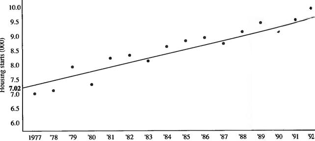
 T=7.02+0.173t.
Figure 8.5 displays the raw data and the trend line they produce.
Given this equation, it is possible to predict the number of housing starts for future time periods merely by substituting the appropriate value for T. Suppose Mayfield Construction wants to forecast the housing starts for 1993. Since the value of T would be 17 in 1993, the forecast becomes
 = 7.02 + 0.173(17) = 9.96.
Or 9,960 starts, since the data were expressed in units of 1,000.

Figure 8.5 – The number of housing starts in Happy Valley and the trend line they produce
Similarly, since 1995 would carry a T value of 19, the forecast for 1995 would be
Y = 7.02 + 0.173(19) = 10.31.
It is estimated that there will be 1,031 housing starts in 1995.
Of course, the farther into the future a forecast is made, the less confidence you can place in its precision. Additionally, its accuracy is based on the condition that the past provides a representative picture of future trends.