090. Moving Averages

A Moving average (MA) will have the effect of “smoothing out” the data, producing a movement with fewer peaks and valleys. It is computed by averaging the values in the time series over a set number of time periods. The same number of time periods is retained for each average by dropping the oldest observation and picking up the newest. Assume that the closing prices for a stock on the New York Stock Exchange for Monday through Wednesday were $20, $22, and $18, respectively. We can compute a three-period (day) moving average as

(20 + 22 + 18) / 3 = 20.

This value of 20 then serves as a forecast or estimate of what the closing price might be at any time in the future. If the closing on Thursday is, say 19, the next moving average is calculated by dropping Monday’s value of 20 and using Thursday’s closing price of 19. Thus, the forecast becomes

(22 + 18 + 19) / 3 = 19.67.

The estimate figured in this manner is seen as the long-run averages of the series. It is taken as the forecast for the closing price on any given day in the future.

Thus, MA: A series of arithmetic averages over a given number of time periods, it is the estimate of the long-run average of the variable.

Example. The sales for Arthur Momitor’s Snowmobiles, Inc., over the past 12 months are shown in Table 8.2. Both a three month MA and a five-month MA are calculated.

Table 8.2 – Snowmobile sales for Arthur Momitor

Month	Sales ($100)	Three-Month MA	Five-Month MA
January	52
February	81	60.00
March	47	64.33	59.00
April	65	54.00	63.20
May	50	62.67	56.00
June	73	56.00	58.60
July	45	59.33	55.60
August	60	51.67	61.40
September	50	63.00	55.80
October	79	58.00	59.20
November	45	62.00
December	62

The first entry in the three-month MA is obtained by averaging the sales of snowmobiles in January, February, and March. The resulting value of (52 + 81 + 47)/3 = 60 is centered on the middle time period of February. The next entry is determined by averaging February, March, and April, and centering the value of 64.33 in the middle of those three periods, which is March. The remaining entries are determined similarly.

The first entry in the five-month MA series uses values for months January through May. The average of (52+51+47+65+50)/5 = 59 is centered in the middle of those five time periods at March.

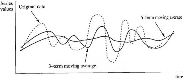
Moving averages have the effect of smoothing out large variations in the data. This smoothing effect occurs because unusually small observations are averaged in with other values, and their impact is thereby restrained. The larger the number of time periods in a moving averageб the more pronounced the smoothing effect will be. Notice that the range of values in the three-month MA is less than that in the original data and greater than the range found in the five-month MA. Figure 8.4 illustrates this tendency for the smoothing effect to increase with the number of time periods in the moving average.

Figure 8.4 – Comparing Moving Averages

Notice that when an odd number of time periods is used in the moving average, the results can be automatically centered at the middle time period. However, if there is an even number of time periods, there is no middle observation at which the value can be automatically centered.

Moving averages can be used to remove irregular and seasonal fluctuations. Each entry in the moving average is derived from four observations of quarterly data – that is, one full year’s worth. Thus, the moving average “averages out” any seasonal variations that might occur within the year, effectively eliminating them and leaving only trend and cyclical variations.

In general, if the number of time periods in a moving average is sufficient to encompass a full year (12 if the monthly data are used; 52 if weekly data are used), seasonal variations are averaged out and removed from the series. The data are then said to be Deseasonalized.

As noted, the use of a larger number of time periods results in a smoother averaged series. Therefore, if the data are quite volatile, a small number of periods should be use in the forecast to avoid placing the forecast too close to the long-run average. If the data do not vary greatly from the long-run mean, a larger number of time periods should be used in forming the moving average.

The moving average method of forecasting is best used when the data show no upward or downward trend. It is a somewhat simplistic approach and finds its most common use in the decomposition of time series.

< Предыдущая		Следующая >