Relationships between variables are either Deterministic or Stochastic (random).
Example 7.2. Deterministic relationship can be expressed by a mathematical model, or formula, that converts speed in miles per hour (mph) into kilometers per hour (kph). Since 1 mile equals approximately 1.6 kilometers, this model is 1 mph = 1.6 kph. Thus, a speed of 5 mph = 5*1.6 = 8.0 kph. This is Deterministic model because there is no error (except for rounding) in the determination of the rate of speed in kph. Given any value for mph, kph can be determined exactly.
Only few relationships in the business world are also exact or so easily determined. In using advertising to determine sales, for Example, there is almost always some variation in the relationship. A model of this nature is said to be Stochastic, due to the presence of random variation. It can be written as
Y = β0 + β1(X) + ε, (7.2)
(deterministic (random
component) component)
Where β0 is the vertical interception of the line; β1 is the slope; ε is a random error term or Disturbance term designed to capture variation above and below the regression line due to all other factors not included in the model (may be positive or negative, depending on whether a value Y, given any X value, lies above or below the regression line).
Thus,
A deterministic mathematical model is expressed as Y = β0 + β1X. Given any value for X, the value of Y can be determined with precision. A stochastic model contains one or more random components that lead to errors in efforts to predict, and is written as Y = β0 + β1(X) + ε.
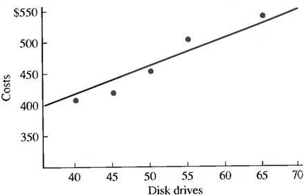
Example 7.3. A computer manufacturer wishes to examine the relationship between the number of hard-disk drivers produced and the total cost. The firm’s head financial analyst and statistician collects data over a five-period for the number of drivers produced and the corresponding costs. Although a sample of only five observations is most likely insufficient, it will serve the purpose of illustration. The data are displayed in Table 7.1. The data are then plotted in a scatter diagram shown in Figure 7.2. If a line is drawn through the middle of the scatter, some observations fall above it while others fall below it. Therefore, not all the observations will fall directly on the regression line. There will likely be some variation above and below it. This deviation above and below the line is reflected in Formula (7.2) by ε.
Table 7.1 - Production data for computer hardware
|
Day |
Number of Drivers |
Cost, $ |
|
1 |
50 |
450 |
|
2 |
40 |
380 |
|
3 |
65 |
540 |
|
4 |
55 |
500 |
|
5 |
45 |
420 |

Figure 7.2 - A scatter diagram for Production Data
To estimate the true population regression line the sample model is used
Y = b0 + b1X + e, (7.2a)
Where B0 - regression constant and B1 – regression coefficient are estimates for the population parameters β0 and β1; e – error component (it usually has a mean value of zero and a variance σ2 of some amount).
The model (7.2a) is then used to estimate the relationship between X and Y, resulting in the regression line
Ŷ = b0 + b1X (7.2b)
Where Ŷ (pronounced Y-hat) – Is the estimated value for the dependent variable and is represented by a point On the regression line.
It should be noticed also that The regression model can be used to predict or forecast the value for the dependent variable.