060. Confidence Intervals for the Population Mean – Small Samples

In the event a small sample (n < 30) must be taken, the normal distribution may not be appropriate. Specifically, when (1) the sample is small and (2) is unknown, the Z-distribution will not apply. Instead, if the population is known to be normal, an alternative distribution, called Student’s t-distribution (or simply the T-distribution) must be used. The Student’s t-distribution was developed in 1908 by William S. Gosset (1876-1937), who worked as a brewmaster for Guinness Breweries in Dublin, Ireland. Guinness would not allow any of its employees to publish their research. When Gosset (who liked to “toy with numbers for pure relaxation”) first reported on the t-distribution, he published under the pseudonym “Student” in order to protect his job. Hence, the term Student’s T-distribution.

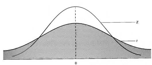
Like the Z-distribution, the t-distribution has a mean of zero, is symmetrical about the mean, and ranges from – ∞ to +∞. However, while the Z-distribution has a variance of 2 = 1, the variance of the T-distribution is greater than l. As a result, the T-distribution is flatter and more dispersed than the Z-distribution (see Figure 6.2).

Figure 6.2 – A Comparison of the T-Distribution and the Z-Distribution

Actually the T-distribution is an entire family of distributions with different variances. The variance of the t-distribution depends on the degrees of freedom (d. f.), which is equal to N – 1.

The variance for the t-distribution can be written as

As n increases, the variance approaches l. When N > 30, the distribution will, like the Z-distribution, have a variance of 1 (or very close to it). This explains why the Z-distribution can be used for large samples.

It is important to remember that the T-distribution is used when

(1) the population is assumed to be normal,

(2) a small sample is taken,

(3) s is unknown.

The T-statistic is calculated like the Z-statistic.

T =

Rewriting (6.3) algebraically a confidence interval for , is

C. I. for = ± (t)(S) = ± T

The proper T-value can be found from Table A. To illustrate, assume you want a 95 percent confidence interval and have a sample of 20 observations. Since N = 20, the degrees of freedom are d. f. = N - 1 = 19. Move down the first column Table F under “d. f.” to 19. Move across that row to the column headed by a confidence level of 0.95 for two-tailed tests. (Ignore the two rows concerning one-tailed tests.) The resulting entry of 2.093 is the proper T-value for a 95 percent confidence interval with a sample size of 20 (d. f. = 19).

Example 6.2 (From a news story in The Wall Street Journal). A construction firm was charged with inflating the expense vouchers it files for construction contracts with the federal government. The contract states that a certain type of job should average $1150. In the interest of time, the directors of only 12 government agencies were called on to enter court testimony regarding the firm’s vouchers. If a mean of $1275 and a standard deviation of $235 are discovered from testimony, would a 95 percent confidence interval support the firm’s legal case? Assume voucher amounts are normal.

A 95 percent level of confidence with d. f. = 12 - 1 = 11 yields from Table A a T-value of 2.201. Then

C. I. for = ± T = 1275 ± (2.201) = 1275 ± 149.31,

$1,125.69 << $1,424.31.

The court can be 95 percent confident that the mean voucher was between $1125 and $1424. Since the interval contains the $1150 amount agreed upon, it would seem to strengthen the firm’s defense.

Example 6.3 (UAW vs FMC). The labor agreement between the United Auto Workers and Ford Motor Company required that the mean output for a particular production section be held at 112 units per month per employee. Disagreement arose between UAW and FMC as to whether this standard was being maintained. The labor agreement specified that if mean production levels dropped below the stipulated amount of = 112, FMC was permitted to take “remedial action”. Due to the cost involved, only 20 workers were tested, yielding a mean of 102 units. Assume a standard deviation of 6.5 units was found and that output levels are normally distributed. Does a 90 percent confidence interval tend to suggest a violation of the labor contract, thereby allowing the remedial action?

Solution:

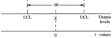
Figure 6.3 – A 90 percent Confidence Interval

With a 90 percent level of confidence and N – 1 = 19 d. f., Table A yields a T-value of 1.729.

C. I. for = ± T = 102 ± (1.729) = 102 ± 3.29,

98.71 < < 105.29.

The mean output level of 112 units specified in the labor contract is not into confidence interval.

Interpretation: There is a 90 percent level of confidence that the contract is being violated. FMC is within its rights to pursue a remedy for lagging productivity.

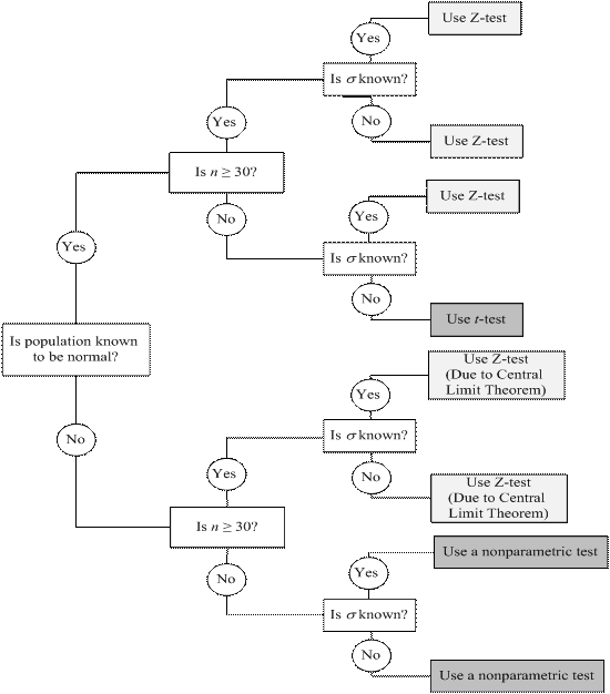
Obviously, deciding whether to use a T-test or a Z-test is crucial. Figure 6.4 will aid in selecting the proper test statistic. Remember that the T-distribution should be used when all three of these conditions are present:

Figure 6.4 - Selecting the Proper Test Statistic for

< Предыдущая		Следующая >