048. Sampling distributions: an introduction to inferential statistics. Introduction

Populations are usually too large to study in their entirety. It is necessary to select a representative sample of a more manageable size. This Sample is then used to Draw conclusions about the population in which statisticians are interested.

Inferential statistics involves the use of a statistic to form a conclusion, or inference, about the corresponding parameter.

The inferential process is extremely important in many statistical analyses. The value of the statistics depends on the sample taken. From any given population of size N, it is possible to get many different samples of size N, i. e. . Each sample may well have a different mean. That is why some sampling error is likely to occur.

The difference between the population parameter (μ) And the sample statistic used to estimate the parameter () is called Sampling error. If a few extremely large observations are drawn for the sample, the sample mean will Overestimate μ. If a few extremely small observations are drawn for the sample, the sample mean will Underestimate μ. The size of the sampling error can never be calculated if the population mean is unknown.

A list of all possible values for a statistic and the probability associated with each value is called a Sampling distribution.

Example 5.1. There is a population N = 4 incomes for four students. These incomes are $100, $200, $300 and $400. The mean income can is μ = $250.

1. There are possible samples of size N = 2 can be selected from this population (see Table 5.1).

2. Each sample has a different mean with exception of the third and fourth samples. The probability of selecting a sample that yields an of 150 is

.

Table 5.1 – All Possible Samples of Size N = 2 from a population of N = 4

Sample	Sample Elements X1	Sample Means
1	100, 200	150
2	100, 300	200
3	100, 400	250
4	200, 300	250
5	200, 400	300
6	300, 400	350

3. If a sample 5 was picked (see Table 5.1), the estimate of μ is = 300, which is greater than the actual value for the population mean. So that, samples 1 and 2 in Table 5.1 produce an underestimate of the population mean.

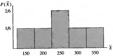
4. Sampling distribution is presented in Table 5.2 and Figure 5.1

Table 5.2 – Sampling Distribution for Samples of Size N = 2 from a Population of N = 4 Incomes

Sample Mean	Number of Samples Yielding	Probability P ()
150	1	1/6
200	1	1/6
250	2	2/6
300	1	1/6
350	1	1/6
Total	-	1

Figure 5.1 - Sampling Distribution for Samples of Size N = 2 from a Population of N = 4 Incomes

< Предыдущая		Следующая >